Authors: Ryan Gengler, Josh Shell, Aaron Verst, Matt Klich
This project sought to explore and visualize the Cincinnati 311 dataset. The 311 non-emergency number is used to report everything from potholes, tenant/landlord issues, sidewalk repair or any other non-emergency city request. Due to the sheer size of the dataset, this team used three months’ worth of data (June – August, n=31,166).
Project Setup
Our work is hosted on a local web application, built on HTML, CSS, and JavaScript. Visualizations were completed using the D3 library, and data manipulation was accomplished through python and excel. To launch the web application, the user can use a simple python server running on LocalHost:XXXX.
Development Process
All work was completed in VS Code, via Live Share so all engineers could work in parallel; at major stopping points all work was backed-up via Git/GitHub. The team used the D3 starter template provided by Dr Aurisano, containing the D3 library. The project folder was then expanded by the addition of
- index.html
- June_August_data2.tsv (dataset)
- Js directory containing 13 .js files which contain the source code for our visualizations and interactions
All front-end interaction is rendered through index.html, after being initialized/called in main.js – their source code for each initialization of each graph is written in their respective .js files. All visualizations are presented using raw values except for days_between. The data was skewed so far left that all other values down the chart were either unreadable or nonsensical; a log scale was used to represent this particular value.
As for the data itself, as mentioned above the team had to only use a sample of the entire dataset due to its size. In regards to raw data, we only had to add two additional columns using basic data science techniques, days_between which calculated the days between the initial call and update, and week_no which told us which week in the calendar year our data belonged to.
Exploration of Graphs and Plots
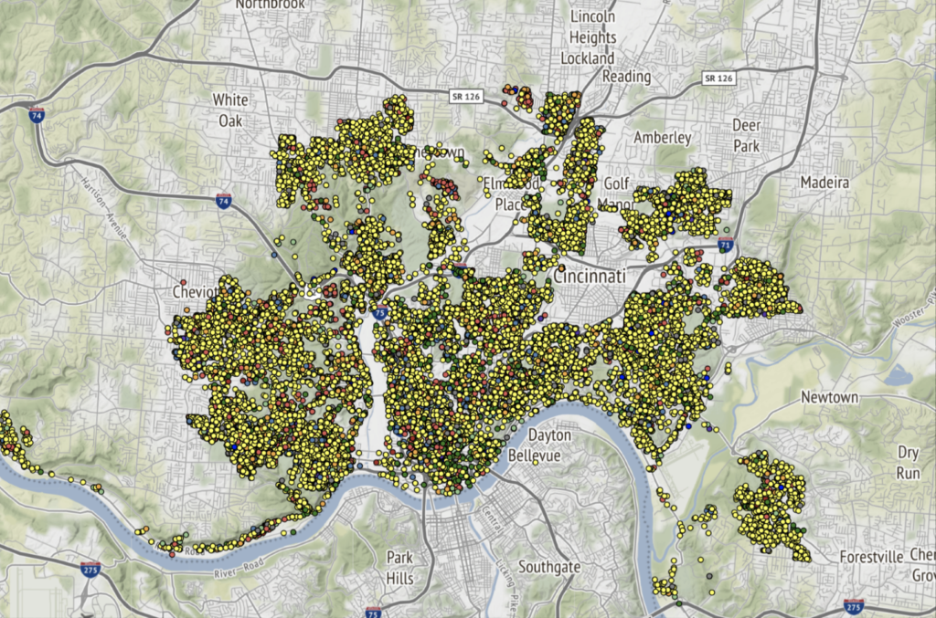
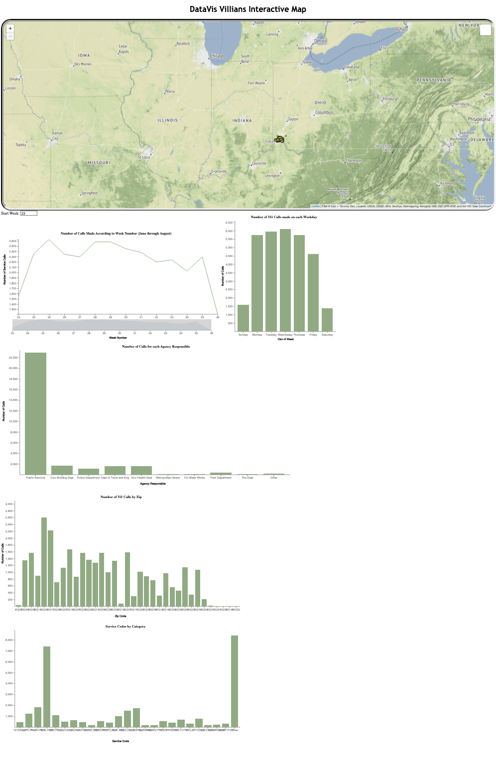
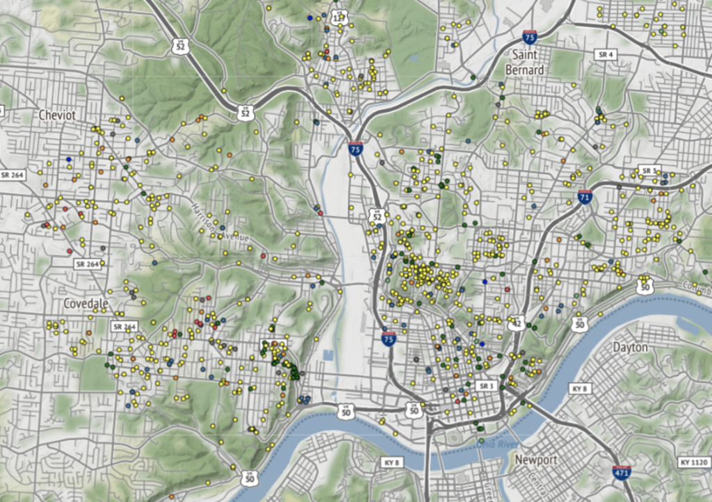
The first visualization is the leaflet map of service calls. Each record in the dataset contained geospatial coordinates, latitude and longitude, and their type of service call. This map is interactive, allowing the user to zoom in/out, change background, hover over specific datapoint, etc.
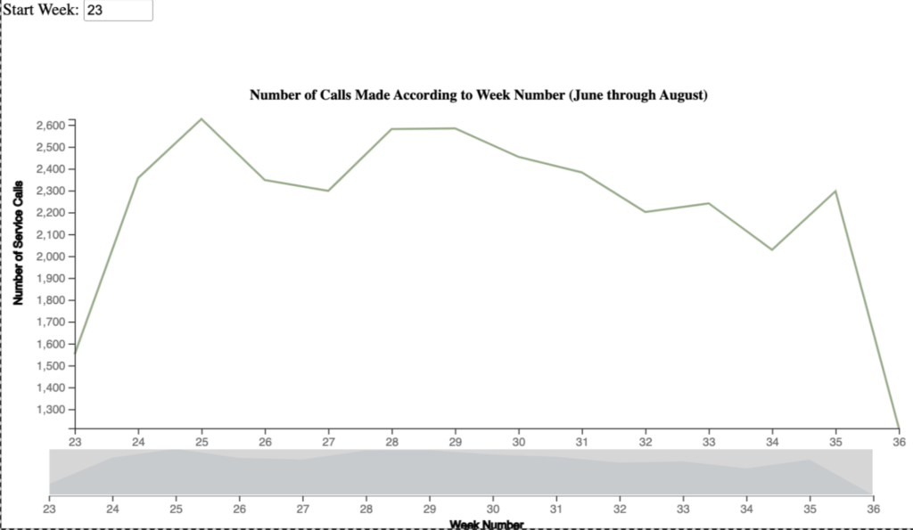
The next chart is a timeline of calls made by week. Due to the sample of the dataset we used, weeks are categorized by their week number for the entire year. In our case, our data runs from calendar week 23 through 36.
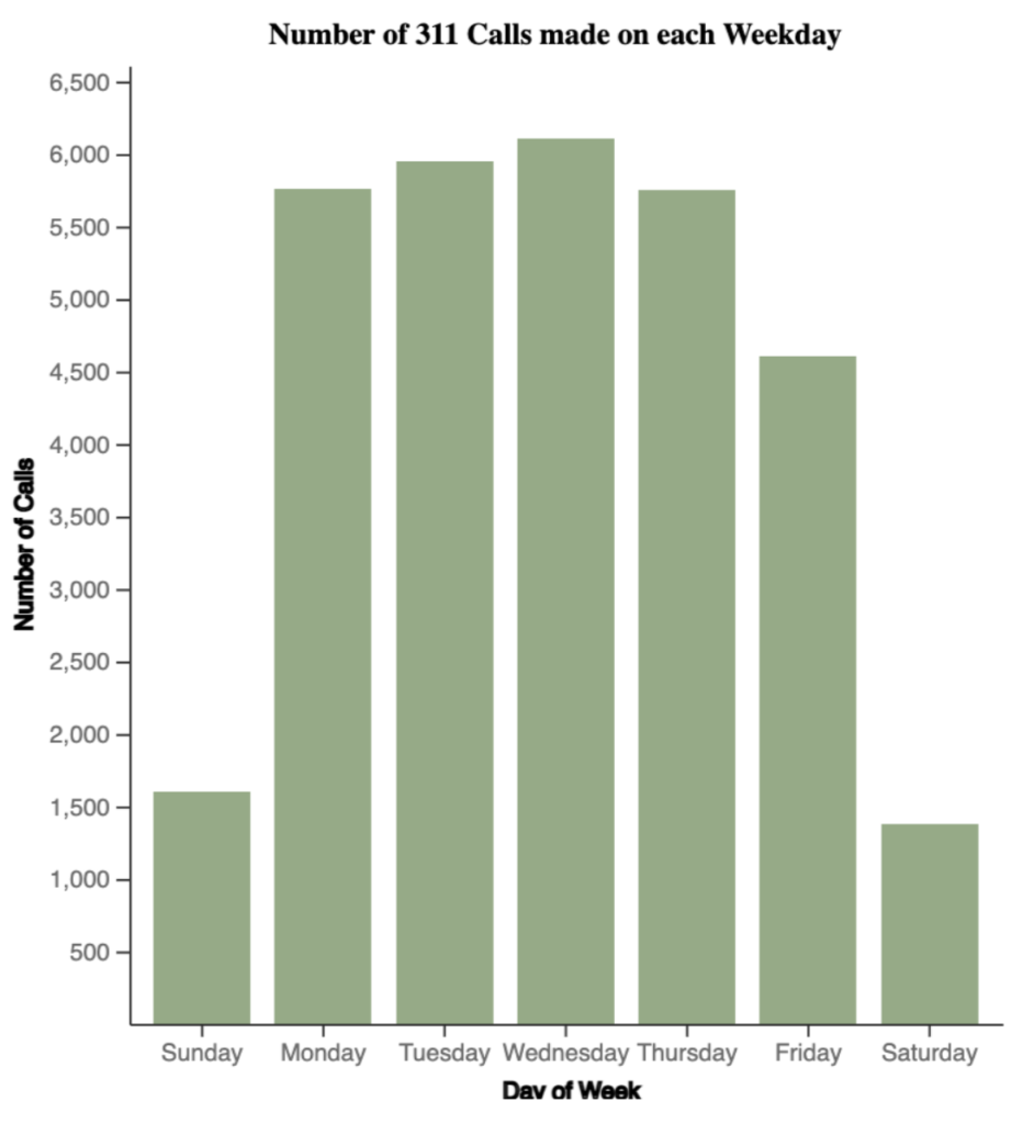
Beside it, is the chart depicting days of the week vs calls made; interestingly there were much fewer calls made on weekends compared to weekdays.
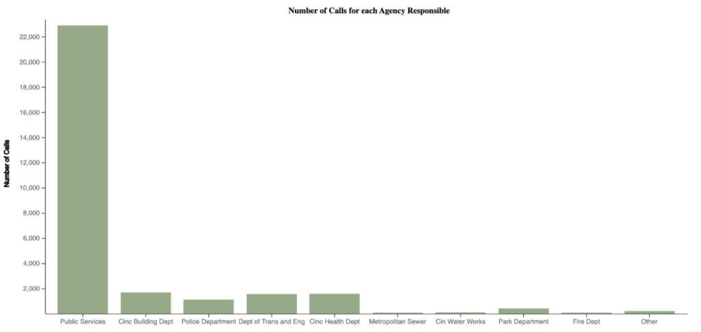
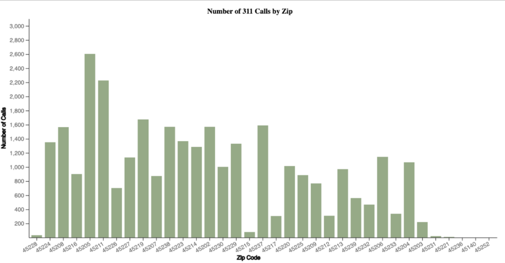
Next, we visualized the number of calls broken down by both the agency responsible for handling the call, and the ZIP code where the call originated.
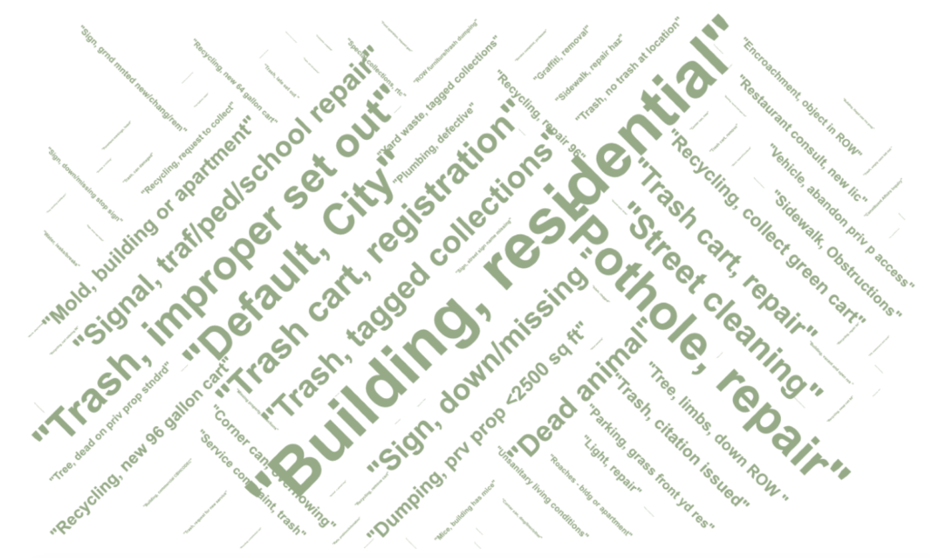
While other graphs and charts can be found on application itself, this group thought the word cloud visualization was an important addition. Given the textual nature of these 311 reports, we wanted to capture what exactly residents were reporting.
Layout
Slide the blue bar above to see the sketch to the final data exploration tool.
Pre-Development Sketches
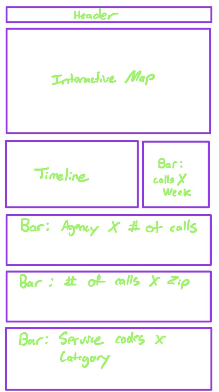
Prior to the finalization of the previously mentioned graphs and plots, we decided on the following layout. The header appears at the top to declare the application’s objective. The interactive map was decided to be the primary tool of significant; therefore, it sits below the header to allow the user to immediately interact. The timeline, to narrow the dataset selection by the date, was the next tool of significance. It therefore sits directly below the tool of interest. The final tools, the bars, were then placed in the best respect to the available screen real-estate.
Post-Development Appearance
As we evaluate the application’s overall appearance post-development, we find some tools were slightly modified or addended. We added a start week box and also added the cloud visualization. The bar charts were also placed based on their needed size for the data at hand.
Findings
After visualizing the data for three summer months, the team noticed some interesting trends. The first being the number of days between an initial service call and its update/response in the system being less than 1 day. Through a word-cloud visualization, we iterated through the body of the requests themselves and pulled out the most commonly used phrases – which happened to be “residential building”, “pothole repair” and variations of “trash” and “collections”. The top 3 ZIP codes where requests were made were 45202, 45211, and 45219; the first of these two are located on the west side of Cincinnati (west of I-75) with 45219 located just north of downtown (Mt. Auburn, Clifton Heights, and Coryville).
Our team was surprised to see many of the calls coming from the West Side of town rather than Downtown or Over the Rhine. What was not surprising were the nature of the calls: potholes, complaints about trash collection, or fallen branches.
Visualization Components
Each visualization on our map is linked, allowing the user to filter through the data. For example, if the user clicks on the Days bar chart they could toggle on and off certain or multiple days. Below, we can see the same map with only Saturday and Sunday calls(top) versus calls placed on all seven days.
Issues
One surface level issue the team faced were the legends for some of the graphs. The number of days and service code bar charts do not have a label on the y-axis. Using the vis.height and vis.width calls the team was unable to properly render these axes like they were able to with other charts. Another issue that we ran into was dealing with the linking between the brush for the timeline and the map. A ton of time was spent on trying to figure that linkage out, but we were never able to figure it out entirely. It works, but the data given back is not always correct.